Easy unsupervised learning demonstration
You can download the original, working jupyter notebook here.
With python, scikit-learn, and handwritten digits.
This is a notebook that I made for a high school student who visited our lab. It is a simple introduction to dimensionality reduction and should not be considered a statement that I’m an expert in unsupervised learning.
Loading the digits dataset
It’s a dataset that contains around 1700 images (8x8 pixels) of handwritten digits. Recognising handwriting is a hard task for a computer, but can nowadays be done with good reliability.
The dataset also contains labels that tell us the ground truth (what digit is contained in each image), but we’re not using them (except at the end, for testing), so this is unsupervised learning. We’ll pretend to only know that there are 10 classes of images (corresponding to 0, 1,…, 9).
import numpy as np
import matplotlib.pyplot as plt
%matplotlib inline
from sklearn.datasets import load_digits

digits_dataset = load_digits()
print(digits_dataset.DESCR)

digits = digits_dataset['images']
n_digits = digits.shape[0]  # how many images are there?
Display an example of these digits
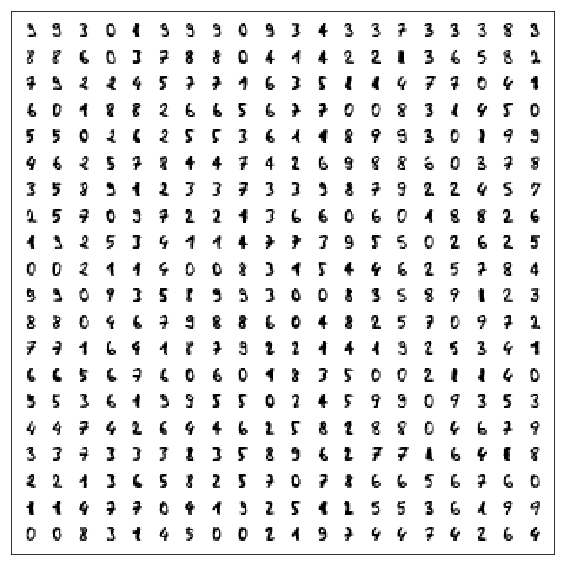
These are some of the images we’re working with.
n = 20
sample_size = n**2
d = 10/n

plt.figure(figsize=(10, 10))
random_sample = np.random.choice(n_digits, replace=False, size=sample_size)
for i in range(sample_size):
    x = i//n
    y = i%n
    plt.imshow(digits[i], cmap=plt.cm.gray_r,
               extent=(x, x+d, y, y+d))

plt.xlim([-.5, 20])
plt.ylim([-.5, 20])
plt.xticks([])
plt.yticks([]);
Dimensionality reduction
Our world is three-dimensional. Mathematically, this means that we need three numbers to identify a point in space: for example the \(x\), \(y\), \(z\) Cartesian coordinates, or, on Earth, latitude, longitude, and altitude.
The “space of digits” is 64-dimensional. What does this mean? Simply, that we need 64 numbers to describe a digit. Each of these number represents a shade of gray for each of the 64 pixels (8x8) of the image.
It’s impossible to visualise 64 dimensions geometrically! So, to put them together, we try to put them in perspective in the same sense as a three dimensional object is drawn on a piece of paper in two dimensions. We try to do this in a clever way that keeps as much information as possible about all the 64 dimensions.
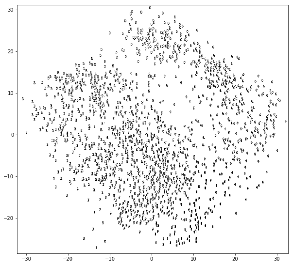
Display the whole dataset with PCA
Principal Component Analysis is a simple algorithm that picks the directions along which there is most variance in the data. We choose to keep the first two only, so that we can draw them down on a plane.
from sklearn.decomposition import PCA

pca_model = PCA(n_components=2)
pca_embedding = pca_model.fit_transform(digits.reshape([-1, 64]))
plt.figure(figsize=(20, 20))
plt.gca().set_aspect('equal')

d = .6
for i in range(n_digits):
    plt.imshow(digits[i], cmap=plt.cm.gray_r,
               extent=(pca_embedding[i, 0],
                       pca_embedding[i, 0]+d,
                       pca_embedding[i, 1],
                       pca_embedding[i, 1]+d))


plt.xlim([pca_embedding[:, 0].min()-1, pca_embedding[:, 0].max()+1])
plt.ylim([pca_embedding[:, 1].min()-1, pca_embedding[:, 1].max()+1]);
Display the whole dataset with t-SNE
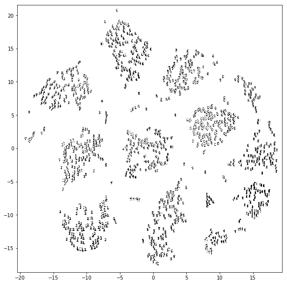
t-SNE (t-distributed stochastic neighbor embedding) is a more sophisticated algorithm which performs dimensionality reduction in a non-linear way, as opposed to PCA which is linear only.
from sklearn.manifold import TSNE

# try playing with perplexity, which is a free parameter
tsne_model = TSNE(perplexity=30.)
tsne_embedding = tsne_model.fit_transform(digits.reshape([-1, 64]))
plt.figure(figsize=(20, 20))
plt.gca().set_aspect('equal')

d = .4
for i in range(n_digits):
    plt.imshow(digits[i], cmap=plt.cm.gray_r,
               extent=(tsne_embedding[i, 0],
                       tsne_embedding[i, 0]+d,
                       tsne_embedding[i, 1],
                       tsne_embedding[i, 1]+d))


plt.xlim([tsne_embedding[:, 0].min()-1, tsne_embedding[:, 0].max()+1])
plt.ylim([tsne_embedding[:, 1].min()-1, tsne_embedding[:, 1].max()+1]);
Clustering with k-means
We can see in the plot above that the dimensionality reduction is so clever that it lumps together images that do look similar to us humans. We just need to identify those clusters and stick a label on them: this group here, we call it “group of 1s”, these others are “the 8s”, and so on.
“Clustering” means finding groups of points that are near each other. There is no reason to limit ourselves to the dimensionality-reduced space above: we can cluster based on the full 64-dimensional space, so that we don’t lose information.
from sklearn.cluster import KMeans

n_classes = 10  # there are 10 digits 0...9

kmeans_model = KMeans(n_clusters=n_classes)
predicted_labels = kmeans_model.fit_predict(digits.reshape([-1, 64]))
plt.figure(figsize=(20, 20))
plt.gca().set_aspect('equal')

for i in range(n_digits):
    plt.imshow(digits[i], cmap=plt.cm.gray_r,
               extent=(tsne_embedding[i, 0],
                       tsne_embedding[i, 0]+d,
                       tsne_embedding[i, 1],
                       tsne_embedding[i, 1]+d))
    plt.imshow([[predicted_labels[i]]], cmap=plt.cm.jet,
               extent=(tsne_embedding[i, 0],
                       tsne_embedding[i, 0]+d,
                       tsne_embedding[i, 1],
                       tsne_embedding[i, 1]+d),
               vmin=0, alpha=.2, vmax=predicted_labels.max())


plt.xlim([tsne_embedding[:, 0].min()-1, tsne_embedding[:, 0].max()+1])
plt.ylim([tsne_embedding[:, 1].min()-1, tsne_embedding[:, 1].max()+1]);
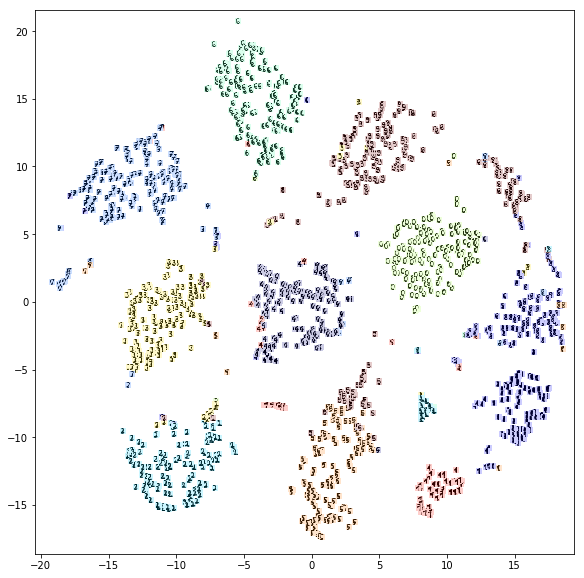
You can see that the colours are consistent in those groups, and each color corresponds more or less to one digits. There are mistakes, of course…
Evaluate performance
We used unsupervised learning. Which means that we didn’t use at all the labels that were provided with the dataset.
Here, I evaluate the performance also using labels: it is evident from the plot above that there is a correspondence between clusters and digits. So we can do a crude thing where we consider “correct” the given labels that coincide with those of the majority of the cluster, and wrong otherwise.
Find what cluster corresponds to which actual digit
true_labels = digits_dataset['target']

consensus_for_cluster = np.empty(n_classes, dtype=int)
for i in range(n_classes):
    digits_in_cluster = predicted_labels == i
    true_labels_cluster = true_labels[digits_in_cluster]
    consensus_for_cluster[i] = np.argmax(np.bincount(true_labels_cluster))
# translate "cluster id" description into "what number is this"
predicted_digits = consensus_for_cluster[predicted_labels]
Measure accuracy
Here we compare to the ground truth.
training_set_accuracy = np.mean(predicted_digits == true_labels)

print("Accuracy on the training set is:", training_set_accuracy, "%")
Accuracy on the training set is: 0.79020589872 %
Is this good or bad?
This is question has a bit of a philosophical answer. Without labels, our algorithm cannot know that we, humans, consider these
 all the same digit. In a context of supervised learning, it could, because we tell it. But here, it can only rely on geometrical similarity. But geometrical similarity would imply that the second of the 1s above might be a slightly tilted 7 instead…
Show example prediction
random_digit = np.random.choice(n_digits)

print("I chose image n.",random_digit, "and it looks as below.")

plt.figure(figsize=(2,2))
plt.imshow(digits[random_digit], cmap=plt.cm.gray_r)
plt.axis('off');

prediction = predicted_digits[random_digit]
truth = true_labels[random_digit]
print("I believe this image contains the digit", prediction)

if prediction==truth:
    print("and it looks like I'm right :D")
else:
    print("but unfortunately the dataset says it's a", truth, ":(")
I chose image n. 1635 and it looks as below.
I believe this image contains the digit 3
and it looks like I'm right :D
